Does the Three-Episode Rule Really Work?

1. The heuristic

Japanese anime is released in seasons. Every three months, thirty to fifty new series begin airing at once, most of them running twelve weekly episodes. A viewer picking up several at the same time has to decide, early and repeatedly, which ones to abandon.

The community’s answer is a rule that nobody wrote down and almost everybody follows: watch the first three episodes, then decide whether to keep going or drop the show. The usual justification is that a series often withholds its real premise until the second or third episode, so a single episode is not enough evidence.

Three is a suspiciously round number for a decision problem, and the rule has a precise structure: a fixed exploration budget per arm, followed by an irrevocable commitment. That is the shape of an Explore-Then-Commit policy. So the number is testable, and this post tests it on real rating data.

2. Formalisation

For one broadcast season, let the arms be the $K$ series airing concurrently. Pulling arm $i$ means watching one episode of series $i$; the reward is the viewer’s satisfaction with that episode, a value in $\{1,\dots,10\}$. Write $\mu_i$ for the true mean quality of series $i$ and $E = 12$ for its episode count.

Under this map the folk rule has the shape of Explore-Then-Commit with $m = 3$: sample every arm $m$ times, then commit to the surviving set for the remaining $E - m$ episodes. The question is whether $m^* = 3$.

Two things are worth separating before going further, because the rest of this post moves between them. ETC describes an allocation — uniform exploration followed by an irrevocable decision. It says nothing about what the decision is for. The folk rule borrows that allocation but serves a different objective from the one ETC is usually analysed against, and §4 makes that objective precise. Under the threshold objective the same uniform-then-commit allocation is what the pure-exploration literature calls uniform allocation; the ETC name is recovered in §6, once a shared budget turns the problem back into cumulative-regret minimisation.

3. Data

All rewards come from bangumi.tv, the largest Chinese-language anime database, via bangumi/Archive [1] — the site’s own periodic data export, published weekly through GitHub Releases specifically so that projects like this one do not have to scrape. Nothing here was crawled; the snapshot used throughout is the dump of 2026-08-18.

The export ships one JSON-lines file per entity type. Only subject.jsonlines is needed here, filtered to type = 2 (anime) and platform = TV. Each record carries the fields an experiment needs to be reproducible — id, name, date, platform, eps, tags, score, rank — and, critically, score_details: the complete one-to-ten rating histogram, not merely an average.

That last field is what makes the study possible without modelling assumptions. Rewards are drawn from the empirical distribution of real votes, so nothing about the arms has to be assumed — not Bernoulli, not Gaussian, not bounded-subgaussian. The per-arm mean and standard deviation used below are simply the moments of that histogram,

$$\mu_i=\frac{1}{N_i}\sum_{v=1}^{10} v\,n_{i,v},\qquad \sigma_i^2=\frac{1}{N_i}\sum_{v=1}^{10}(v-\mu_i)^2 n_{i,v},$$

with $n_{i,v}$ the number of votes of value $v$ and $N_i=\sum_v n_{i,v}$. Series with fewer than 100 votes are excluded; each season is restricted to its ten most-voted titles, which is roughly the number a single viewer would actually consider.

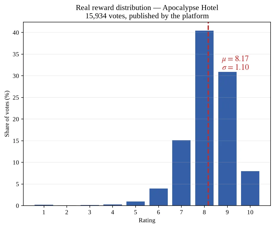
Fig. 1. The reward distribution of a single arm, taken directly from the published vote histogram. The mass is concentrated and left-skewed, and nothing about its shape was chosen.

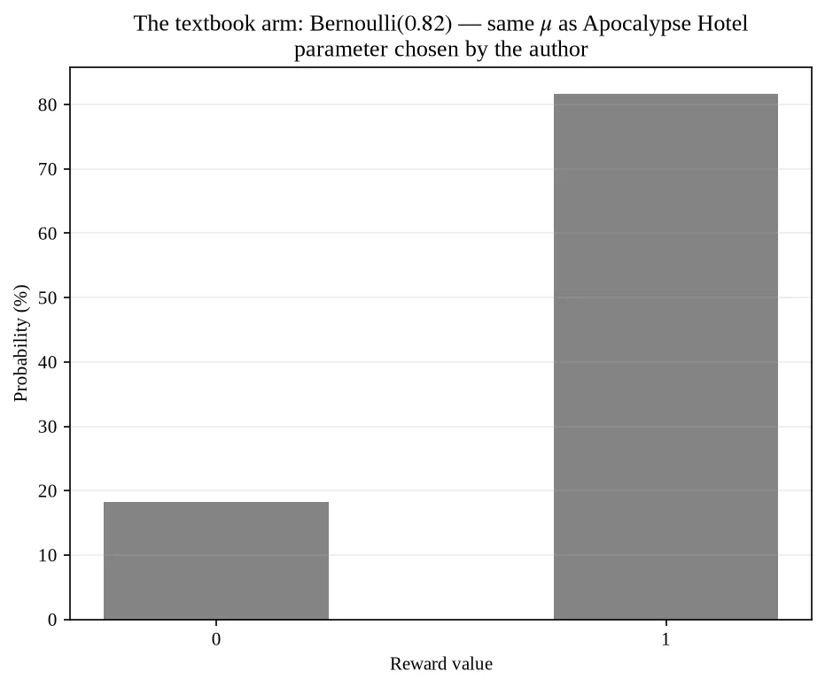
Fig. 2. The textbook substitute: a Bernoulli arm with the same mean. It matches $\mu_i$ by construction and misrepresents everything else, including the variance that determines how many episodes a decision needs.

4. The objective is a threshold test, not best-arm identification

Classical MAB asks for $\arg\max_i \mu_i$. That is not what a viewer wants. The question is not which of a season’s shows is best, but whether each show, taken on its own, is good enough. The model therefore fixes a personal bar $\theta$ — say $\theta = 7$ out of 10 — and evaluates every arm against $\theta$ rather than against the other arms.

This is a change of objective, not of algorithm: the allocation is still uniform-then-commit, but what it is trying to get right is a per-arm classification rather than a maximisation. The setting is close to the Thresholding Bandit Problem (TBP) of Locatelli et al. [2], a fixed-budget pure-exploration problem in which the learner must return the set of arms whose means lie above a known threshold $\tau$, up to a precision $\varepsilon$. Their difficulty measure is

$$\Delta_i := |\mu_i - \tau| + \varepsilon, \qquad H := \sum_{i=1}^{K}\Delta_i^{-2},$$

and their algorithm, APT (Anytime Parameter-free Thresholding), attains a matching upper and lower bound on the probability of misclassification — a 0–1 criterion over the returned set. The uniform-sampling baseline it is measured against is called Uniform Allocation (UA), which is precisely the allocation the folk rule performs.

Two things separate the present setting from theirs.

Mistakes are not equally expensive. APT is judged on whether the returned set is right at all, so every misclassification counts the same. Here the cost of a mistake scales with the gap: keeping a show far below the bar wastes more time than keeping one that barely misses it. The objective is therefore a weighted loss rather than an error probability.

The two error directions are asymmetric. Watching additional episodes of a show above the bar costs nothing — exploration and exploitation coincide on good arms. The only losses are (a) time spent on a show below the bar, and (b) the forfeited enjoyment of a good show dropped too early. There is no symmetric “regret of over-exploration” on the good side at all.

Making this precise: after $m$ episodes the sample mean of arm $i$ has standard error $s_i = \sigma_i/\sqrt{m}$, and by the CLT the probability of each misclassification is a normal tail. Writing $d_i = \mu_i - \theta$, the expected season loss is

$$L(m)=\underbrace{\sum_{i:\,d_i<0}(-d_i)\Big[\,m+(E-m)\,\Phi\!\big(d_i/s_i\big)\Big]}_{\text{time wasted on shows below the bar}}\;+\;\underbrace{\sum_{i:\,d_i>0}d_i\,(E-m)\,\Phi\!\big(-d_i/s_i\big)}_{\text{enjoyment lost by dropping good shows}}$$

where $\Phi(d_i/s_i) = \Pr[\bar X_i \ge \theta]$ is the chance a below-bar show still looks acceptable after $m$ episodes, and $\Phi(-d_i/s_i)$ is the chance an above-bar show still looks unacceptable. The first term grows in $m$ (screening is itself expensive); the second falls in $m$ (more evidence, fewer good shows discarded). The optimum is

$$m^* = \arg\min_{1\le m\le E} L(m).$$

Note that $m$ is a single number shared by the whole season, not chosen per show. That constraint is not an approximation for tractability — it is what the folk rule actually is.

5. What the optimum turns out to be

For Spring 2025 at $\theta = 7$, the two terms cross and the total is minimised at $m^* = 2$.

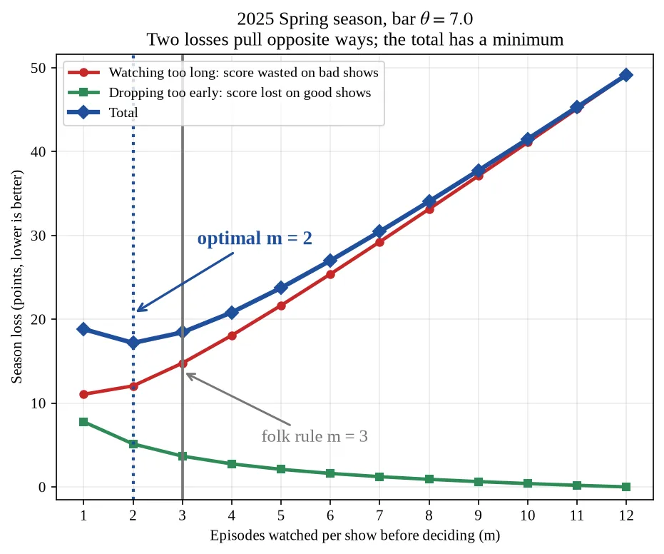
Fig. 3. The two terms of $L(m)$ pull in opposite directions. Time wasted on shows below the bar rises with $m$; enjoyment lost to premature drops falls with it. The total has an interior minimum, here at $m^* = 2$, one episode earlier than the folk rule.

Run over the fourteen most recent seasons, $m^*$ always lands between 1 and 3, and where it lands is determined by the bar. At a demanding bar the optimum moves earlier: the gaps $\Delta_i$ are larger for most arms, each episode is more informative, and less screening is needed. At a relaxed bar of $\theta = 6.5$ the optimum is exactly three, in six of the fourteen seasons.

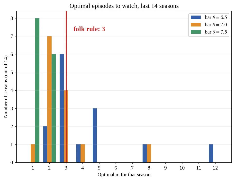
Fig. 4. $m^*$ computed independently for each of the last fourteen seasons, at three values of the bar. The optimum never leaves $\{1,2,3\}$, and the bar alone decides where inside that range it falls.

So the folk number is not arbitrary. It is the correct answer for a viewer who is easy to please, and it sits at the boundary of the optimal range for everyone else. What the community got wrong is not the number but its universality: three is a solution to one instance of the problem, presented as a solution to all of them.

6. Reintroducing the shared budget

The model so far has a structural gap. Each show is screened independently, its losses summed; nothing forces the arms to compete. Real viewing is not like that. Ten interesting shows at twelve episodes each is 120 episodes, roughly forty-eight hours in a three-month window, and few people have forty-eight hours to spend this way.

Imposing a shared budget $B \ll KE$ restores the classical bandit: the arms now compete for a scarce resource, exploration genuinely trades off against exploitation, and the folk rule becomes one policy among several that can be compared on regret against the best-arm benchmark. This is also where the ETC label becomes exact rather than merely descriptive — the objective is now cumulative regret, which is what ETC is normally analysed against, so putting it beside UCB1 and Thompson Sampling is a fair comparison rather than an analogy. Crucially, the screening is paid for out of $B$ — running the folk rule with $m = 3$ over ten shows consumes 30 episodes before any exploitation begins.

Budget	Thompson Sampling	Folk rule ($m=3$)
$B = 40$ (tight)	16.1	24.6
$B = 80$ (loose)	13.5	17.1

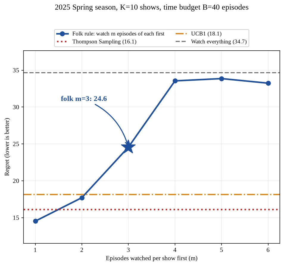
Fig. 5. Tight budget, $B = 40$. Screening ten shows for three episodes each consumes 30 of the 40 available, leaving almost nothing for exploitation, and the adaptive policies separate clearly.

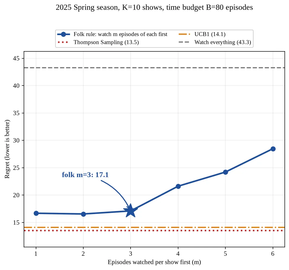
Fig. 6. Loose budget, $B = 80$. The same fixed screening cost is now a quarter of the budget rather than three quarters, and the gap narrows sharply.

At $B = 80$, watching everything without filtering loses 43.3 by the same measure, so every policy here beats no policy at all.

The pattern is that the folk rule’s disadvantage is a function of scarcity. At $B = 40$ its fixed screening cost consumes three quarters of the budget and it loses badly. At $B = 80$ it has room to exploit what it found and closes most of the gap. The rule quietly assumes its user is not especially short of time — an assumption that is invisible in the rule as stated, and false for exactly the viewers who most need a filtering heuristic.

7. Putting regret back on the ten-point scale

Cumulative regret over a season is awkward to interpret: 16.1 is not obviously good or bad. Since the reward is already a score out of ten, the natural rescaling is to divide by the budget. If a policy accumulates reward $R$ over $B$ episodes, its mean satisfaction per episode is $R/B$, and regret converts directly:

$$\frac{R_{\text{policy}}}{B} \;=\; \frac{R_{\text{oracle}}}{B} \;-\; \frac{\mathrm{Regret}}{B}.$$

At $B = 40$ the oracle collects 7.733 per episode, so Thompson Sampling’s regret of 16.1 is a shortfall of $16.1/40 = 0.40$ points per episode, putting it at 7.33. Every quantity below is on that scale, and the whole comparison becomes a ladder:

	Score per episode
Best single show, $\mu_{\max}$	8.17	not reachable at this budget
Oracle at $B = 40$	7.73	the benchmark regret is measured against
Thompson Sampling	7.33	best of the policies compared
No filtering, watch all 120	6.88	$=\overline{\mu}$

Reading the gaps in order:

• 6.88 → 7.33 = 0.45. What filtering an entire season actually buys.
• 7.33 → 7.73 = 0.40. What a policy with perfect knowledge of every $\mu_i$ would gain on top. This is the real headroom left to any algorithm.
• 7.73 → 8.17 = 0.44. Unreachable at any budget, and not an algorithmic failure at all: the best show only has twelve episodes, so 28 of the 40 must come from lower-rated shows however well they are chosen.

The distance from the best algorithm to $\mu_{\max}$ is 0.85 points, but roughly half of it is structural rather than learnable — an artefact of a season being made of twelve-episode shows. The honest statement is the middle row: after all the filtering, a perfectly informed viewer would still beat the best algorithm by 0.40 points per episode, which is about the same size as everything filtering achieved in the first place.

So the algorithms capture roughly half of what is available to them, and every one of them lands inside the same narrow band. A gap that all algorithms share, and that persists against an oracle with the same budget, is not an algorithmic problem. It is a property of the reward model, and the remainder of this post is about where it comes from.

8. Direction 1: the reward model assumes a single shared taste

Every reward above was sampled from the public histogram. That embeds a strong assumption: that all viewers draw satisfaction from the same distribution, so that a show’s quality is a scalar property of the show. Under that assumption there is very little left for a bandit to discover — the ranking of the arms is already published on the website, and any policy that reads it starts at the optimum. This explains both the small size of the filtering gain and the failure of UCB1 and Thompson Sampling to separate from a fixed-$m$ rule: there is almost no information to acquire.

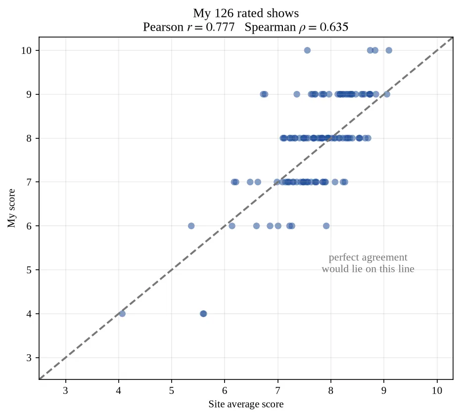
Fig. 7. One viewer’s ratings against the site average, over 126 shows. Agreement on the raw scale hides substantial disagreement in the ordering, which is the only thing a bandit policy consumes.

A single-viewer check gives the size of the effect. Across 126 shows rated by one viewer (the author), agreement with the site average is $r = 0.777$ on raw scores. But a bandit policy never uses raw scores — it uses the induced ordering, and there Spearman’s $\rho$ falls to $0.64$. Nineteen percent of those ratings differ from consensus by a full point or more, with a mean absolute deviation of 0.65.

One viewer establishes only that the discrepancy exists, not its distribution. The site publishes each user’s own rating list, and collecting those at scale is a tooling problem that is already solved: bgm-cli [3], a Node command-line client for Bangumi, reads subjects, users and per-user collections and emits JSON for direct use in an analysis pipeline. Extending the study over many viewers is therefore a question of sampling and consent rather than of engineering.

9. Direction 2: creators have a track record

The second direction starts from an observation about the arms themselves. A new series is not an unknown object: its studio, director, composer and writer have almost always made other shows, and those shows are already rated.

Exploiting this within a season would place the problem in the correlated-bandit framework of Gupta et al. [4]. There, pulling arm $k$ and observing reward $r$ yields a pseudo-reward

$$s_{\ell,k}(r)\;\ge\;\mathbb{E}\big[R_\ell \mid R_k = r\big]$$

which bounds every other arm and lets non-competitive arms be eliminated after $O(1)$ pulls instead of $O(\log T)$.

Within a season the data does not support that route. Core creative roles are almost never shared — across the seasons examined, at most 2 of 45 same-season pairs share a director, writer or composer, for the obvious reason that one director cannot run two productions at once.

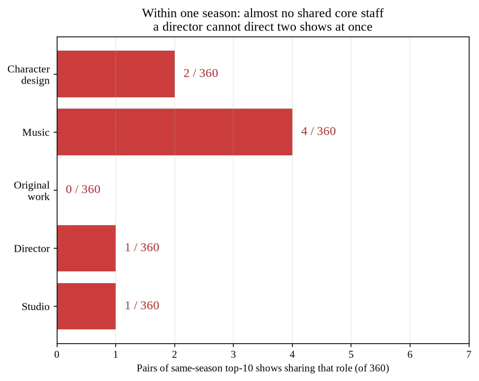
Fig. 8. Shared core creative roles between concurrently airing shows. There is essentially nothing to borrow inside one season, which is what rules out the correlated-arm route in its literal form.

Widen the window and the structure is abundant. Of 80 shows examined, 78 have at least one earlier release from the same studio and 65 have one from the same director, with a median of 29 prior same-studio titles.

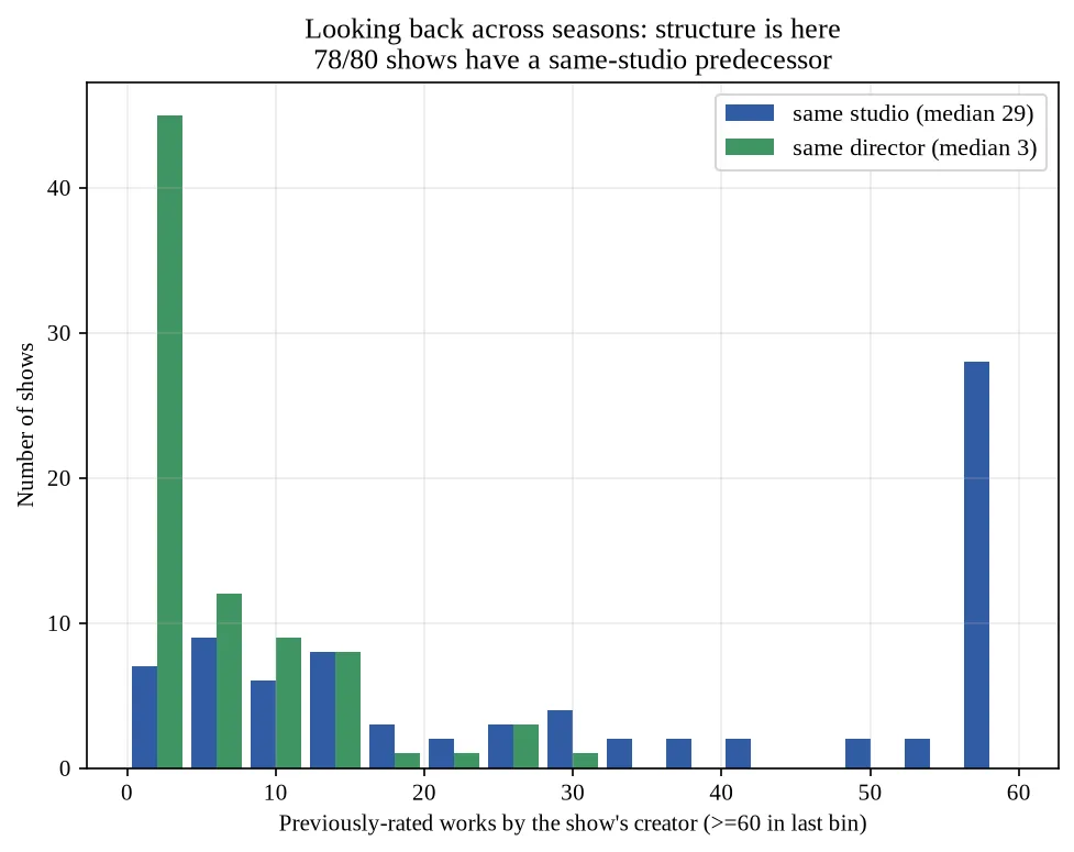
Fig. 9. Counting backwards instead: how many earlier releases each show shares a studio or a director with. The distribution is dense, and it is entirely observed before the season opens.

But those earlier shows are not arms in the current run. They are already-observed history, fully rated before the season begins. Nothing is learned about them by pulling; no information travels between concurrent arms. This is therefore not arm-to-arm correlation. It is a prior on a new arm, and it changes a different quantity: it does not alter $\Delta_i = |\mu_i - \theta|$, but it reduces the number of episodes needed to resolve the sign of $\Delta_i$.

The natural home for it is a linear bandit. Let $x_i \in \mathbb{R}^d$ encode the production features of series $i$ — studio, director, writer, composer — and let $\beta$ be the viewer’s taste vector over those features, shared across all arms and all seasons:

$$\mathbb{E}[r_{i,t}] = \langle x_i,\, \beta\rangle .$$

A viewer’s rating history is a set of observations of $\beta$, not of any particular arm. A new series is then a new feature vector rather than a new unknown, and a LinUCB-style policy inherits the whole back catalogue as a warm start. This also unifies the two directions: $\beta$ is precisely “individual taste” from §8, given a parametric form.

Both routes require the same thing that this study did not have — per-viewer joint ratings rather than aggregate histograms. A pseudo-reward table has to be estimated from viewers who rated both arms; a taste vector $\beta$ has to be fit per viewer. That is the next measurement, and the only real prerequisite for either direction.

10. Summary

• The three-episode rule is a uniform-then-commit allocation, which makes it testable rather than merely repeatable. Whether that allocation is called uniform allocation or ETC depends on the objective it is serving, and the two objectives appear at different points in this analysis.
• The right objective is a threshold test against a personal bar, with an asymmetric, gap-weighted loss — close to the Thresholding Bandit Problem [2], but scored by a weighted loss rather than by probability of misclassification.
• Under that loss the optimum is $m^* \in \{1,2,3\}$, determined by the bar. Three is correct for an undemanding viewer and too slow for everyone else.
• Once a shared time budget is imposed, the rule’s fixed screening cost makes it clearly worse than UCB1 or Thompson Sampling when time is scarce, and nearly competitive when it is not.
• On a per-episode scale, filtering a season buys 0.45 points, a perfectly informed viewer at the same budget would gain only 0.40 more, and a further 0.44 is structurally out of reach because each show has just twelve episodes. Every algorithm lands in the same narrow band, which points at the reward model rather than at the policies.
• Modelling taste as a per-viewer parameter over production features turns the back catalogue into a prior and places the problem in the linear-bandit setting.

The parsing, analysis and plotting code is on GitHub. It reads the official archive directly, so every number and figure above can be reproduced from the snapshot named in [1].

1. 三话定律是什么

日本动画按季度播出。每三个月，三十到五十部新番同时开播，绝大多数是十二集的周更。一个同时追好几部的观众，必须反复地、而且是尽早地决定：哪些接着看，哪些放弃。

圈子里的答案是一条没人写下来、却几乎人人遵守的规矩：先看三话，再决定是追下去还是弃掉。通常的理由是，一部番往往要到第二或第三话才交出真正的设定，只看一话证据不足。

对一个决策问题来说，“三”是个可疑地整齐的数字。而这条规矩的结构非常明确：每条臂固定探索若干次，然后做出不可撤销的承诺，这正是 Explore-Then-Commit（先探索后承诺，下称 ETC）策略的形状。既然如此，这个数字就可以被检验。

2. 写成老虎机问题

取一个播出季度，把当季同时开播的 $K$ 部番作为臂（arm）。拉动臂 $i$ 表示看一集第 $i$ 部番，奖励是观众对这一集的满意度，取值在 $\{1,\dots,10\}$。记 $\mu_i$ 为第 $i$ 部番的真实平均质量，$E = 12$ 为集数。

在这个映射下，三话定律具有 $m = 3$ 的 ETC 形状：每条臂采样 $m$ 次，然后对留下来的臂在剩余 $E - m$ 集里执行到底。问题是 $m^*$ 是否真的等于 3。

有两件事需要先分开，因为后文会在两者之间来回移动。ETC 描述的是一种分配方式（allocation）：均匀探索，然后不可撤销地决定。它并不规定这个决定是为了什么。三话定律借用了这个分配方式，但它服务的目标（objective）和 ETC 通常被分析时所针对的目标不同，第 4 节会把这个目标写清楚。在阈值目标下，同样的”先均匀采样再承诺”在纯探索文献里叫均匀分配（Uniform Allocation, UA）；ETC 这个名字要到第 6 节、共享预算把问题变回累积遗憾最小化时，才重新变得严格。

3. 数据从哪来

所有奖励来自 bangumi.tv，中文圈最大的动画数据库，经由 bangumi/Archive [1] 获取。那是站方自己的定期数据导出，每周通过 GitHub Releases 发布，目的正是让这类项目不必去爬站。本文没有抓取任何数据，全程使用的是 2026-08-18 那一次快照。

该导出按实体类型各给一个 JSON-lines 文件。这里只用到 subject.jsonlines，筛选条件为 type = 2（动画）且 platform = TV。每条记录都带着复现实验所需的字段：id、name、date、platform、eps、tags、score、rank，以及最关键的 score_details，也就是完整的一到十分评分直方图，而不只是一个平均分。

正是最后这个字段让整项研究免于建模假设。奖励直接从真实投票的经验分布中采样，因此不需要对臂做任何参数假定，伯努利、高斯、有界次高斯都不用。下文用到的每条臂的均值与标准差，就是该直方图的矩：

$$\mu_i=\frac{1}{N_i}\sum_{v=1}^{10} v\,n_{i,v},\qquad \sigma_i^2=\frac{1}{N_i}\sum_{v=1}^{10}(v-\mu_i)^2 n_{i,v},$$

其中 $n_{i,v}$ 是打 $v$ 分的票数，$N_i=\sum_v n_{i,v}$。投票数少于 100 的作品被剔除；每个季度只取投票数最高的十部，这大致就是一个观众实际会考虑的数量。

图 1. 单条臂的奖励分布，直接取自公开的投票直方图。质量集中且左偏，其形状不是任何人选定的。

图 2. 教科书里的替身：一条与之同均值的伯努利臂。它按构造对上了 $\mu_i$，却错报了其余的一切，包括决定”判断需要几集”的那个方差。

4. 判的是每部番够不够线

经典多臂老虎机要找的是 $\arg\max_i \mu_i$。但观众要的不是这个。真正的问题是每一部番单独拿出来，够不够得上标准。为此，模型设定一条个人标准线 $\theta$，比如十分制下的 7 分，然后拿每条臂去和 $\theta$ 比，不和其他臂比。

换掉的是目标，不是算法：分配方式仍然是先均匀采样再承诺，只是它要做对的事情从”最大化”变成了”逐臂分类”。这个设定接近 Locatelli 等人 [2] 的 Thresholding Bandit Problem（TBP），一个固定预算的纯探索问题，学习者需要在精度 $\varepsilon$ 之内，返回均值高于已知阈值 $\tau$ 的那些臂。其难度度量为

$$\Delta_i := |\mu_i - \tau| + \varepsilon, \qquad H := \sum_{i=1}^{K}\Delta_i^{-2},$$

他们提出的算法 APT（Anytime Parameter-free Thresholding）在误判概率这一指标上取得了相互匹配的上下界，那是一个针对返回集合的 0–1 判据。它所对照的均匀采样基线，原文就称为 Uniform Allocation（UA），而这恰恰就是三话定律所执行的那种分配方式。

本文的设定与之有两处不同。

判错的代价不相等。 APT 衡量的是返回集合对不对，因此每一次误判都一样重。而在这里，代价随间隔放大：留下一部远低于标准线的番，比留下一部只差一点点的番，浪费的时间更多。这里的目标因此是一个加权损失，不是一个误判概率。

两个方向的错误不对称。 对一部高于标准线的番，多看几集完全不花代价，在好的臂上探索和利用是同一件事。真正的损失只有两种：花在低于标准线的番上的时间，以及过早弃掉一部好番所放弃的享受。在好的一侧，根本不存在”探索过度”这种对称的遗憾。

把它写精确。看过 $m$ 集之后，臂 $i$ 的样本均值标准误为 $s_i = \sigma_i/\sqrt{m}$，由中心极限定理，两类误判的概率都是正态尾概率。记 $d_i = \mu_i - \theta$，则整季的期望损失为

$$L(m)=\underbrace{\sum_{i:\,d_i<0}(-d_i)\Big[\,m+(E-m)\,\Phi\!\big(d_i/s_i\big)\Big]}_{\text{浪费在低于标准线的番上的分数}}\;+\;\underbrace{\sum_{i:\,d_i>0}d_i\,(E-m)\,\Phi\!\big(-d_i/s_i\big)}_{\text{因过早弃番而丢掉的分数}}$$

其中 $\Phi(d_i/s_i) = \Pr[\bar X_i \ge \theta]$ 是一部低于标准线的番在 $m$ 集之后看上去仍然合格的概率，$\Phi(-d_i/s_i)$ 则是一部高于标准线的番在 $m$ 集之后看上去仍然不合格的概率。第一项随 $m$ 递增，因为筛选本身要花时间；第二项随 $m$ 递减，因为证据更多、误弃更少。最优解为

$$m^* = \arg\min_{1\le m\le E} L(m).$$

这里的 $m$ 是整季共用的一个数字，不是逐番选择的。这个约束不是为了求解方便而做的近似，三话定律本来就是这样一条规矩。

5. 最优的 m 是几

在 2025 年春季、$\theta = 7$ 的设定下，两项损失在中间交叉，总和的最小值落在 $m^* = 2$。

图 3. $L(m)$ 的两项朝相反方向拉扯。浪费在低于标准线的番上的时间随 $m$ 上升，因过早弃番丢掉的享受随 $m$ 下降。总和存在内部极小，此处为 $m^* = 2$，比民间规矩早一集。

把它放到最近十四个季度上跑，$m^*$ 始终落在 1 到 3 之间，而具体落在哪里，只取决于那条线的高低。标准越严，最优点越靠前：此时大多数臂的间隔更大，每一集携带的信息量更高，需要的筛选就更少。而在 $\theta = 6.5$ 这样一条宽松的线上，最优解恰好就是三，十四个季度里有六个落在这里。

图 4. 对最近十四个季度分别独立计算的 $m^*$，取三种标准线。最优值从未离开 $\{1,2,3\}$，而落在这个区间的哪一点，只由标准线决定。

所以这个民间数字并不是凭空来的。对一个要求不高的观众，三就是正确答案；对其余人，它也停在最优区间的边缘上。圈子搞错的是它的普适性：三是这个问题某一个实例的解，却被当成了所有实例的解。

6. 加上时间预算之后

到这里为止，模型有一个结构性的缺口。每部番各自筛选、损失各自累加，没有任何东西迫使这些臂互相竞争。而真实的观看不是这样：十部感兴趣的番、每部十二集，就是 120 集，在三个月里大约四十八小时，很少有人拿得出这四十八小时。

加上一个共享预算 $B \ll KE$，经典的老虎机问题就回来了：臂现在要争夺一项稀缺资源，探索与利用之间产生了真正的取舍，三话定律也就成了若干可比策略中的一个，可以在”对最优臂的遗憾”这个尺度上被衡量。这里也正是 ETC 这个称呼从描述性变为严格的地方：目标现在是累积遗憾，而这正是 ETC 通常被分析的对象，所以把它和 UCB1、Thompson Sampling 摆在一起比较是公平的，不是打个比方。

另外有一点很关键：筛选本身是从 $B$ 里出的。用 $m = 3$ 跑十部番，在开始利用之前就已经消耗了 30 集。

时间预算	Thompson Sampling	三话定律（$m=3$）
$B = 40$（紧）	16.1	24.6
$B = 80$（松）	13.5	17.1

图 5. 紧预算，$B = 40$。十部番各筛三集就要吃掉 40 集里的 30 集，几乎不剩利用的余地，自适应策略因此明显拉开。

图 6. 松预算，$B = 80$。同样的固定筛选开销现在只占四分之一而不是四分之三，差距迅速收窄。

在 $B = 80$ 下，完全不筛选、把 120 集全看完，在同一尺度上损失 43.3。所以任何策略都好过没有策略。

规律是：三话定律的劣势是稀缺程度的函数。在 $B = 40$ 时，它固定的筛选开销吃掉了四分之三的预算，输得很难看；在 $B = 80$ 时，它有余地去利用筛出来的结果，差距被抹平了大半。

这条规矩默默假设了它的使用者并不特别缺时间。 这个假设在规矩的表述里完全看不见，而且恰恰对那些最需要筛选启发式的观众不成立。

7. 把遗憾换算成每集得分

整季的累积遗憾本身不好读：16.1 究竟算好还是算差，看不出来。既然奖励本来就是十分制的分数，自然的换算就是除以预算。若某策略在 $B$ 集里累计奖励 $R$，则它的每集平均满意度为 $R/B$，而遗憾可以直接换算：

$$\frac{R_{\text{policy}}}{B} \;=\; \frac{R_{\text{oracle}}}{B} \;-\; \frac{\mathrm{Regret}}{B}.$$

$B = 40$ 时先知每集拿到 7.733 分，因此 Thompson Sampling 那 16.1 的遗憾就是每集少 $16.1/40 = 0.40$ 分，落在 7.33。下面所有数字都在这个尺度上，整个比较变成一道阶梯：

	每集得分
最好的单部番，$\mu_{\max}$	8.17	该预算下不可达
$B = 40$ 的先知	7.73	遗憾真正对照的基准
Thompson Sampling	7.33	参与比较的策略中最好的
完全不筛选，120 集全看	6.88	$=\overline{\mu}$

逐段来读这几个差距：

• 6.88 → 7.33 = 0.45。 筛选整整一季实际买到的东西。
• 7.33 → 7.73 = 0.40。 一个完全知道每个 $\mu_i$ 的策略还能额外拿到的部分。这才是留给任何算法的真实空间。
• 7.73 → 8.17 = 0.44。 任何预算下都拿不到，而且根本不是算法的失败：最好那部番只有十二集，所以 40 集里必有 28 集得从评分更低的番里出，无论怎么选都一样。

最后这一行值得留意，因为那个醒目的数字很容易被误读。最好的算法距离 $\mu_{\max}$ 是 0.85 分，但其中大约一半是结构性的，不是可学习的，它只是”一季由十二集的番构成”这一事实的产物。诚实的说法是中间那一行：在所有筛选之后，一个完全知情的观众也只比最好的算法每集多拿 0.40 分，而这与筛选本身买到的 0.45 分差不多大。

所以算法拿到了可及范围里的大约一半，而且每一个都落在同一条窄带里。一道所有算法共有、并且在同等预算的先知面前依然存在的差距，指向的是奖励模型，本文剩下的部分就是在追问它从哪来。

8. 出路一：口味不是所有人共享的

上面每一个数字，都是从公共直方图里采样出来的。这里嵌着一个很强的假设：所有观众的满意度服从同一个分布，因而”质量”是番本身的一个标量属性。在那个世界里，老虎机几乎无事可做，因为臂的排序早就公布在网站上了，任何读一眼排行榜的策略都从最优点出发。这同时解释了两件事：筛选带来的收益为什么这么小，以及 UCB1 和 Thompson Sampling 为什么拉不开与固定 $m$ 的差距。可获取的信息本来就所剩无几。

图 7. 一位观众在 126 部番上的评分与站点均分的对照。原始分数上的一致掩盖了排序上的大量分歧，而排序恰恰是老虎机策略唯一消费的东西。

用单个观众的数据可以看出这种偏离有多大。以某一位观众（本文作者）评过分的 126 部番为例，与站点均分在原始分数上的相关为 $r = 0.777$。但老虎机策略从不使用原始分数，它使用的是由分数诱导出的排序，而在排序上，Spearman 相关降到了 $\rho = 0.64$。其中 19.0% 的评分与大众相差一整分以上，平均绝对偏差为 0.65 分。

一个人只能说明这种偏离存在，说明不了它的分布。而这个站点会公开每个用户自己的评分列表，把它们批量取回在工具层面已经解决了：bgm-cli [3] 是一个 Node 写的 Bangumi 命令行客户端，可以读取条目、用户与逐用户收藏，并输出 JSON 直接进入分析管线。把研究推广到多用户，剩下的是采样与授权的问题。

9. 出路二：创作者的往绩可以当先验

第二个方向从臂本身的性质出发。一部新番并不是一个未知的物体：它的制作公司、导演、音乐、脚本几乎总是做过别的作品，而那些作品早就被打过分了。

若要在同一季度内部利用这一点，问题就会落进 Gupta 等人 [4] 的相关臂框架。在那里，拉动臂 $k$ 并观测到奖励 $r$ 之后，可以给出伪奖励（pseudo-reward）

$$s_{\ell,k}(r)\;\ge\;\mathbb{E}\big[R_\ell \mid R_k = r\big]$$

它为其余每条臂给出上界，使得非竞争臂只需 $O(1)$ 次拉动即可淘汰，而不是 $O(\log T)$ 次。

但在季度内部，数据不支持这条路。核心创作岗位几乎从不重合：在考察的各季度中，同季 45 个配对里最多只有 2 对共享导演、脚本或音乐，原因很直白，一个导演没法同时带两部片。

图 8. 同期播出的番之间核心创作岗位的重合。一季内部基本无可借用，这正是相关臂那条路在字面意义上走不通的原因。

把窗口放宽，结构立刻变得稠密。在考察的 80 部番中，78 部至少有一部同公司的前作，65 部有同导演的前作，同公司前作数量的中位数是 29 部。

图 9. 反过来往回数：每部番与多少部更早的作品共享公司或导演。分布相当稠密，而且这些信息在开季之前就已经全部被观测到了。

问题在于，那些前作并不是本轮的臂。它们是已经观测完毕的历史，在这一季开始之前就已经全部有分。拉臂不会让人对它们知道得更多，也没有任何信息在同期的臂之间流动。所以这是新臂上的先验（prior），不是臂间相关。 它改变的也是另一个量：它不改变 $\Delta_i = |\mu_i - \theta|$，它减少的是判定 $\Delta_i$ 符号所需要的集数。

它天然的归宿是线性老虎机（linear bandit）。令 $x_i \in \mathbb{R}^d$ 编码第 $i$ 部番的制作特征，包括公司、导演、脚本、音乐；再令 $\beta$ 为这位观众在这些特征上的口味向量，跨所有臂、所有季度共享：

$$\mathbb{E}[r_{i,t}] = \langle x_i,\, \beta\rangle .$$

这样一来，一位观众的历史评分就是对 $\beta$ 的一组观测，而不是对某一条具体臂的观测。一部新番于是只是一个新的特征向量，LinUCB 一类的策略可以把整个片库当作热启动。

这个形式还把两个方向合并了：$\beta$ 正是第 8 节说的”个人口味”，只不过给了它一个参数形式。

两条路都需要同一样本研究没有的东西：逐用户的联合评分，而不是聚合直方图。伪奖励表必须由”同时评过两条臂”的用户估计出来；口味向量 $\beta$ 必须逐用户拟合。这是下一步要做的测量，也是两个方向唯一真正的前置条件。

10. 小结

• 三话定律是一种”先均匀采样再承诺”的分配方式，因而它可以被检验。至于它该叫均匀分配还是 ETC，取决于它服务的目标，而这两个目标在本文的不同位置出现。
• 正确的目标是对一条个人标准线的阈值判定，损失是不对称的、按间隔加权的。这接近 Thresholding Bandit Problem [2]，但它的判据是加权损失，而非误判概率。
• 在这个损失下，最优解是 $m^* \in \{1,2,3\}$，由那条线决定。三对一个要求不高的观众是对的，对其他所有人都太慢。
• 一旦加上共享的时间预算，固定的筛选开销会让它在时间紧张时明显劣于 UCB1 和 Thompson Sampling，而在时间宽裕时接近持平。
• 换算到每集得分：筛选一季买到 0.45 分，同等预算下完全知情的观众也只能再多拿 0.40 分，另有 0.44 分因为每部番只有十二集而结构性地不可达。所有算法都落在同一条窄带里，这指向奖励模型。
• 把口味建模成制作特征上的逐用户参数，可以把整个片库变成先验，并把问题放进线性老虎机的框架。

解析、分析与画图的代码在 GitHub 上。它直接读官方归档，所以上文每一个数字和每一张图都能从 [1] 里那份快照复现。

References

[1] Bangumi, “bangumi/Archive: periodic data export of bangumi.tv.” [Online]. Available: https://github.com/bangumi/Archive. Weekly release, Wednesdays 05:00 GMT+8. Snapshot used: dump-2026-08-18, file subject.jsonlines.
[2] A. Locatelli, M. Gutzeit, and A. Carpentier, “An optimal algorithm for the thresholding bandit problem,” in Proc. 33rd Int. Conf. Machine Learning (ICML), New York, NY, USA, 2016, vol. 48, pp. 1690–1698.
[3] Aronnax, “bgm-cli: a command-line client for Bangumi,” AGPL-3.0. [Online]. Available: https://github.com/aronnaxlin/bgm-cli
[4] S. Gupta, S. Chaudhari, G. Joshi, and O. Yağan, “Multi-armed bandits with correlated arms,” IEEE Trans. Inf. Theory, vol. 67, no. 10, pp. 6711–6732, Oct. 2021, doi: 10.1109/TIT.2021.3081508.